1. Model Overview

DVMDOSTEM is designed to simulate the key biophysical and biogeochemical processes between the soil, the vegetation and the atmosphere. The evolution and refinement of DVMDOSTEM have been shaped by extensive research programs and applications both in permafrost and non-permafrost regions ([Genet et al., 2013]; [Genet et al., 2018]; [Jafarov et al., 2013]; [Yi et al., 2010]; [Yi et al., 2009]; [Euskirchen et al., 2022]; [Briones et al., 2024]). The model is spatially explicit and represents ecosystem response to climate and disturbances at seasonal (i.e. monthly) to centennial scales. The snow and soil columns are split into a dynamic number of layers to represent their impact on thermal and hydrological dynamics and the consequences for soil C and N dynamics. Vegetation composition is modeled using community types (CMTs), each of which consists of multiple plant functional types (PFTs - groups of species sharing similar ecological traits). This structure allows the model to represent the effect of competition for light, water and nutrients on vegetation composition [Euskirchen et al., 2009], as well as the role of nutrient limitation on permafrost ecosystem dynamics, with coupling between C and N cycles ([McGuire et al., 1992]; [Euskirchen et al., 2009]). Finally, the model represents the effects of wildfire in order to evaluate the role of climate-driven fire intensification on ecosystem structure and function([Yi et al., 2010]; [Genet et al., 2013]). The structure of DVMDOSTEM is represented visually in Fig. 1.1 .

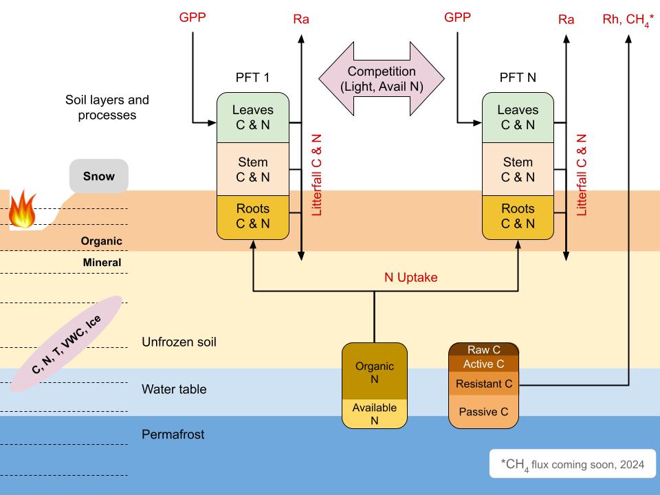
Fig. 1.1 Overview of DVMDOSTEM soil and vegetation structure. On the left is the soil structure showing the layers and different properties that are tracked (purple bubble: carbon (C), nitrogen (N), temperature (T), volumetric water content (VWC), ice). Each of the layers with properties described above is also categorized as organic (fibric or humic) or mineral. Additionally, the model simulates snow layers and the removal of soil organic layers due to fire. On the right is the vegetation structure showing plant functional types (PFTs) within a community type (CMT) and the associated pools and fluxes of C and N. Each PFT is split into compartments (leaf, stem and root) which track their own C and N content and associated fluxes. The fluxes are represented with red text while the pools are black. In addition, there is competition among the PFTs for light, water, and available N, shown with the purple arrow in the top center.

1.1. Structure

DVMDOSTEM is multi-dimensional. It operates across spatial and temporal dimensions, soil layers, and plant functional types.

Fig. 1.2 DVMDOSTEM is a spatially explicit. The base unit of computation is a pixel. There pixels are laid out in a grid. Each pixel is run based on the status of a run mask, which is one of the required input files. Each pixel is parameterized for both soil and vegetation properties. Together the parameterizaton values define a Community Type (CMT). Each pixel is modeled using Plant Functional Types (PFTs) and a layer stack for soil and snow.

1.1.1. Spatial

DVMDOSTEM can be applied at the site level or across large regions. Spatially, DVMDOSTEM breaks up the landscape into grid cells, each of which is characterized by a set of input forcing and parameterization values. Gridded parameterization values describe soil and vegetation characteristics associated with each Community Type (CMT). DVMDOSTEM does not include the lateral transfer of information between grid cells. The CMT classification for each grid cell is static across the time dimension of a model simulation. These two factors limit the ability of the model to represent climate-driven biome shifts or succession trajectories from disturbances such as wildfire [Johnstone et al., 2010]. Design discussions are in progress for adding these capabilities to DVMDOSTEM.

DVMDOSTEM itself is agnostic to the spatial resolution - the resolution is controlled by the input files provided. Recent work has been done with 1km spatial resolution.

1.1.2. Temporal

DVMDOSTEM is a temporal model: a run consists of executing the ecologic processes through consecutive time-steps. Much of the modeling is occurring at a monthly time step, although some process execute at a daily resolution and some processes are yearly.

To initialize historical or future simulations, DVMDOSTEM needs to compute a quasi steady-state (QSS) solution. This solution is forced by using averaged historical atmospheric and ecosystem properties (e.g. soil texture) to drive the model. QSS of physical processes (e.g. soil temperature and water content) are usually achieved in less than 100 years, while QSS of biogeochemical processes (e.g. soil and vegetation \(C\) and \(N\) stocks) are achieved in 1,000 to >10,000 years. However, to decrease overall run-times, DVMDOSTEM uses two QSS stages: “Pre-run” and “Equilibrium”. The list of all DVMDOSTEM run stages is as follows:

• Pre-run (pr): QSS computation for the physical state variables.

• Equilibrium (eq): QSS computation for the biogeochemical state variables.

• Spinup (sp): introduction of pre-industrial climate variability and fire regime.

• Transient (tr): historical simulation.

• Scenario (sc): future simulation.

Model simulation requires advancing the model consecutively through all of the run stages as needed (pr -> eq -> sp -> tr ->). It is possible to work with any subset of the stages using the command line --restart flag.

Note

Automatic equilibrium (QSS) detection.

DVMDOSTEM does not have an internal test for whether or not equilibrium (quasi steady state; QSS) has been reached. In other words, if you specify --max-eq=20000, the model will run for 20,000 years no matter what internal state it reached. It appears that some of the variable and constant names and the command line flag --max-eq are vestigial remains of an attempt at “automatic equilibrium detection”.

pre-run (pr)

The pre-run is an equilibrium run for the physical variables of the model. It is typically 100 years, uses constant climate (typically monthly average computed from the [1901-1930] period).

equilibrium (eq)

In the equilibrium stage, the climate is fixed. That is, the climate does not vary from year to year. There will be intra-annual variability to represent the seasons, but from year to year the calculations will be carried out using the same annual cycles. Equilibrium run stage is used in the calibration mode, and is typically the first stage run for any complete simulation. During the eq stage, the annual climate inputs used are actually calculated as the mean of the first 30 years of the historic climate dataset (specified in the config file), so the mean of the values from 1901-1930.

spinup (sp)

In the spinup stage, the climate is not fixed: the driving climate is used from the first 30 years of the historic climate dataset. Should the spstage be set to run longer than 30 years, the 30 year climate period is re-used. In the sp stage the fire date is fixed, occuring at an interval equal to the Fire Recurrence Interval (FRI).

transient (tr)

In the transient stage, the climate varies from year to year. The tr stage is used to run the model over the period of historical record. The input climate data for the tr stage should be the historic climate. This is typically the climate data for the 20th century, so roughly 1901-2009.

scenario (sc)

In the scenario stage, the climate also varies from year to year, but rather than observed variability, a predicted climate scenario is used.

1.1.3. Community Types (CMTs)

Each DVMDOSTEM grid cell can be assigned one “community type” (CMT). A community type is essentially a parameterization that specifies many properties for vegetation, and soil.

1.1.4. Vegetation Types (PFTs)

Each vegetation CMT (e.g. “wet-sedge tundra”, “white spruce forest”, etc.), is modeled with up to ten PFTs (e.g., “deciduous shrubs”, “sedges”, “mosses”), each of which may have up to three compartments: leaf, stem, and root. Vegetation \(C\) and \(N\) fluxes are calculated at each time step based on environmental factors and soil properties. Assimilation of atmospheric \(CO_2\) by the vegetation is estimated by computing gross primary productivity (GPP) for each PFT. GPP is a function of foliage development (seasonal and successional patterns), air and soil temperature, water and nutrient availability, photosynthetically active radiation, and maximum assimilation rate (a calibrated parameter) ([McGuire et al., 1992]; [Euskirchen et al., 2009]). Changes in vegetation \(C\) stocks are calculated using GPP, autotrophic respiration (Ra), and litter-fall (transfer from vegetation to soil). Vegetation \(N\) stocks are calculated using plant \(N\) uptake and litter-fall. Vegetation \(C\) and \(N\) stocks may also be modified as a result of wildfire burn.

1.1.5. Soil and Snow (Layers)

The soil column is structured as a sequence of layers organized by soil horizons (i.e. fibric, humic, mineral, and parent material). The number and physical properties of layers may change throughout the simulation based on vegetation, thermal, hydrologic, and seasonal properties that are calculated at each time step ([Zhuang et al., 2003]; [Euskirchen et al., 2014]; [Yi et al., 2009]; [McGuire et al., 2018]). The model uses the two-directional Stefan algorithm to predict freezing/thawing fronts and the Richards equation to predict soil moisture dynamics in the unfrozen layers ([Yi et al., 2009]; [Yi et al., 2010]; [Zhuang et al., 2003]). Snow is also represented with a dynamic stack of layers. The physical properties of the snowpack (density, thickness, and temperature) are calculated from snowfall, sublimation and snowmelt. Snow cover influences soil-thermal and hydrological seasonal dynamics. Changes in soil \(C\) stocks are a result of litter-fall from the vegetation and decomposition of soil \(C\) stocks by microbes (heterotrophic respiration or Rh). Changes in soil organic and available \(N\) stocks are a result of litter-fall, net mineralization of organic \(N\) , and plant \(N\) uptake. Soil organic layers and soil \(C\) and \(N\) stocks may also be modified due to wildfire.

1.2. Inputs/Outputs (IO)

NetCDF files [Rew and Davis, 1990] are used as model inputs and outputs, conforming to the CF Conventions v1.11 [Eaton et al., 2011] where possible.

1.2.1. Inputs

The input variables used to drive DVMDOSTEM include: drainage classification (upland or lowland), CMT classification, topography (slope, aspect, elevation), soil texture (percent sand, silt, and clay), climate (air temperature, precipitation, vapor pressure, incoming shortwave radiation), atmospheric \(CO_2\) concentration, and fire occurrence (date and severity). All input datasets are spatially explicit, except the time series of atmospheric \(CO_2\).

Generally TEM requires several types of inputs:

• Spatially explicit - varies over spatial dimensions.

  Examples are the topography variables, slope, aspect and elevation, which change for geographic location, but are fixed through time.

• Temporally explicit - varies over time dimension.

  An example (and in fact the only such input for TEM) is atmospheric CO2 concentration, which is roughly the same across the globe, but varies over time.

• Temporally and spatially explicit - varies over time and spatial dimensions.

  Examples are climate variables like air temperature and precipitation.

The dvmdostem code is neither particularly smart nor picky about the input files. There is minimal built-in error or validity checking and the program will happily run with garbage input data or fail to run because of an invalid attribute or missing input data value. It is up to the user to properly prepare and validate their input data. There is a helper program specifically for generating inputs from data provided by SNAP. This data was prepared as part of the Alaska IEM project (more info here). It remains an open project to generate input data from another source, e.g. ERA5 or a different soil database, etc.

Here some things that are generally assumed (program will likely run; results will likely be invalid) or expected (program unlikely to run if condition not met) of dvmdostem input files:

• The model assumes the dimension order to be (time, Y, X), as per CF Conventions.

• The time axes of the files are assumed to align exactly.

• Input file spatial extents are assumed to align exactly.

• The model expects inputs in NetCDF format.

• The variables names are expected to exactly match the names as shown in the table below.

While there is full support for geo-referenced files, this is not a requirement. Internally, the model requires the latitude for only a single calculation. The geo-referencing information is simply passed along to the output files. It is not used internally and is primarily for provenance and to enable pre and post processing steps. In the event that the file(s) are projected and or geo-referenced, they should contain extra variables and attributes for projection coordinate data, unprojected coordinate data, and grid mapping strings.

The complete list of required TEM input variables is shown below.

file	variable name	dimensions	units
run-mask.nc
	run	Y X
drainage.nc
	drainage_class	Y X
vegetation.nc
	veg_class	Y X
topo.nc
	slope	Y X
	aspect	Y X
	elevation	Y X
soil-texture.nc
	pct_sand	Y X
	pct_silt	Y X
	pct_clay	Y X
co2.nc projected-co2.nc
	co2	year
historic-climate.n c projected-climate. nc
	tair	time Y X	celcius
	precip	time Y X	mm month-1
	nirr	time Y X	W m-2
	vapor_press	time Y X	hPa
	time	time	days since YYYY-MM-DD HH:MM:SS
fri-fire.nc
	fri	Y X
	fri_severity	Y X
	fri_jday_of_bur n	Y X
	fri_area_of_bur n	Y X
historic-explicit- fire.nc projected-explicit -fire.nc
	exp_burn_mask
	exp_jday_of_bur n
	exp_fire_severit y
	exp_area_of_bur n
	time	time	days since YYYY-MM-DD HH:MM:SS

Note

Example code to generate the above table.

import os; import netCDF4 as nc
indir_path = "demo-data/cru-ts40_ar5_rcp85_ncar-ccsm4_toolik_field_station_10x10"
for f in filter(lambda x: '.nc' in x, os.listdir(indir_path)):
    ds = nc.Dataset(os.path.join(indir_path, f))
    print(f)
    for vname, info  in ds.variables.items():
        if 'units' in info.ncattrs():
            us = info.units
        else:
            us = ''
        print("  {:25s},{:15s},{:25s}".format( vname, ' '.join(info.dimensions),us))

1.2.2. Outputs

There are approximately 110 different variables available for output from DVMDOSTEM. One file will be produced per requested output variable. Users can specify the temporal and structural resolutions at which model outputs are produced. This functionality allows users to consider their computational resources and information needs when setting up a model run.

The outputs that are available for DVM-DOS-TEM are listed in the config/output_spec.csv file that is shipped with the repo. The following table is built from that csv file:

Hint

Wide table, scroll right to see all columns!

Table 1.1 output_spec.csv

Name	Description	Units	Yearly	Monthly	Daily	PFT	Compartments	Layers	Data Type	Placeholder
ALD	Soil active layer depth	m		invalid	invalid	invalid	invalid	invalid	double
AVLN	Total soil available N	g/m2			invalid	invalid	invalid		double
BURNAIR2SOILN	Nitrogen deposit from fire emission	g/m2/time			invalid	invalid	invalid	invalid	double
BURNSOIL2AIRC	Burned soil C	g/m2/time			invalid	invalid	invalid	invalid	double
BURNSOIL2AIRN	Burned soil N	g/m2/time			invalid	invalid	invalid	invalid	double
BURNTHICK	Ground burn thickness	m			invalid	invalid	invalid	invalid	double
BURNVEG2AIRC	Burned vegetation C to atmosphere	g/m2/time			invalid	invalid	invalid	invalid	double
BURNVEG2AIRN	Burned vegetation N to atmosphere	g/m2/time			invalid	invalid	invalid	invalid	double
BURNVEG2DEADC	Burned vegetation C to standing dead C	g/m2/time			invalid	invalid	invalid	invalid	double
BURNVEG2DEADN	Burned vegetation N to standing dead N	g/m2/time			invalid	invalid	invalid	invalid	double
BURNVEG2SOILABVC	Burned vegetation C to soil above	g/m2/time			invalid	invalid	invalid	invalid	double
BURNVEG2SOILABVN	Burned vegetation N to soil above	g/m2/time			invalid	invalid	invalid	invalid	double
BURNVEG2SOILBLWC	Burned vegetation C to soil below	g/m2/time			invalid	invalid	invalid	invalid	double
BURNVEG2SOILBLWN	Burned vegetation N to soil below	g/m2/time			invalid	invalid	invalid	invalid	double
CMTNUM	Community Type Number	m		invalid	invalid	invalid	invalid	invalid	int
DEADC	Standing dead C	g/m2			invalid	invalid	invalid	invalid	double
DEADN	Standing dead N	g/m2/time			invalid	invalid	invalid	invalid	double
DEEPC	Amorphous SOM C	g/m2			invalid	invalid	invalid	invalid	double
DEEPDZ	Amorphous SOM horizon thickness	m		invalid	invalid	invalid	invalid	invalid	double
DRIVINGNIRR	Input driving NIRR	W/m2	invalid	invalid		invalid	invalid	invalid
DRIVINGRAINFALL	Input driving precip data after being split from snowfall	mm				invalid	invalid	invalid	float
DRIVINGSNOWFALL	Input driving precip data after being split from rainfall	mm				invalid	invalid	invalid	float
DRIVINGTAIR	Input driving air temperature data	degree_C	invalid	invalid		invalid	invalid	invalid	float
DRIVINGVAPO	Input driving vapor pressure	hPa	invalid	invalid		invalid	invalid	invalid	float
DWDC	Dead woody debris C	g/m2/time			invalid	invalid	invalid	invalid	double
DWDN	Dead woody debris N	g/m2/time			invalid	invalid	invalid	invalid	double
EET	Actual ET	mm/m2/time					invalid	invalid
FRONTSDEPTH	Depth of fronts	mm				invalid	invalid		double
FRONTSTYPE	Front types					invalid	invalid		int
GPP	GPP	g/m2/time	y		invalid			invalid	double
GROWEND	Growing ending day	DOY		invalid	invalid	invalid	invalid	invalid	int
GROWSTART	Growing starting day	DOY		invalid	invalid	invalid	invalid	invalid	int
HKDEEP	Hydraulic conductivity in amorphous horizon	mm/day				invalid	invalid	invalid	double
HKLAYER	Hydraulic conductivity by layer	mm/day			invalid	invalid	invalid	forced	double
HKMINEA	Hydraulic conductivity top mineral	mm/day				invalid	invalid	invalid	double
HKMINEB	Hydraulic conductivity middle mineral	mm/day				invalid	invalid	invalid	double
HKMINEC	Hydraulic conductivity bottom mineral	mm/day				invalid	invalid	invalid	double
HKSHLW	Hydraulic conductivity in fibrous horizon	mm/day				invalid	invalid	invalid	double
INGPP	GPP without N limitation	g/m2/time			invalid			invalid	double
INNPP	NPP witout N limitation	g/m2/time			invalid			invalid	double
INNUPTAKE	Unlimited N uptake by plants. N uptake by happy plants when N is not limited.	g/m2/time			invalid		invalid	invalid	double
IWCLAYER	IWC by layer	m3/m3			invalid	invalid	invalid	forced	double
LAI	LAI	m2/m2			invalid		invalid	invalid	double
LAYERDEPTH	Layer depth from the surface	m			invalid	invalid	invalid	forced	double
LAYERDZ	Thickness of layer	m			invalid	invalid	invalid	forced	double
LAYERTYPE	0:moss 1:shlw 2:deep 3:mineral				invalid	invalid	invalid	forced	int
LTRFALC	Litterfall C	g/m2/time			invalid			invalid	double
LTRFALN	Litterfall N	g/m2/time			invalid			invalid	double
LWCLAYER	LWC by layer	m3/m3			invalid	invalid	invalid	forced	double
MINEC	Mineral SOM C	g/m2			invalid	invalid	invalid	invalid	double
MOSSDEATHC	Moss death carbon	g/m2			invalid	invalid	invalid	invalid	double
MOSSDEATHN	Moss death nitrogen	g/m2			invalid	invalid	invalid	invalid	double
MOSSDZ	Moss thickness	m		invalid	invalid	invalid	invalid	invalid	double
NDRAIN	N losses from drainage (AVLN)	g/m2/time	invalid	invalid	invalid	invalid	invalid	invalid	double
NETNMIN	Soil net N mineralization	g/m2/time			invalid	invalid	invalid		double
NIMMOB	Nitrogen immobilization	g/m2/time			invalid	invalid	invalid		double
NINPUT	N inputs into soil (AVLN)	g/m2/time			invalid	invalid	invalid	invalid	double
NLOST	N losses from soil (AVLN)	g/m2/time			invalid	invalid	invalid	invalid	double
NPP	NPP	g/m2/time			invalid			invalid	double
NRESORB	NRESORB	??			invalid			invalid	double
NUPTAKELAB	Labile N uptake by plants	g/m2/time			invalid		invalid	invalid	double
NUPTAKEST	Structural N uptake by plants	g/m2/time			invalid			invalid	double
ORGN	Total soil organic N	g/m2			invalid	invalid	invalid		double
PERCOLATION	Percolation by layer		invalid	invalid		invalid	invalid	forced	double
PERMAFROST	Permafrost (1 or 0)			invalid	invalid	invalid	invalid	invalid	int
PET	Potential ET	mm/m2/time					invalid	invalid	double
QDRAINAGE	Water drainage quotient (~ratio)				invalid	invalid	invalid	invalid	double
QDRAINLAYER	Qdrain per layer	mm	invalid	invalid		invalid	invalid	forced	double
QINFILTRATION	Water infiltration quotient (~ratio)				invalid	invalid	invalid	invalid	double
QRUNOFF	Water runoff quotient (~ratio)				invalid	invalid	invalid	invalid	double
RAINFALL	Total rainfall	mm			invalid	invalid	invalid	invalid	double
RECO	Summed ecosystem respiration	g/m2/time			invalid	invalid	invalid	invalid	double
RG	Growth respiration	g/m2/time			invalid			invalid	double
RHDWD	Dead woody debris HR	g/m2/time			invalid	invalid	invalid	invalid	double
RHSOM	Heterotrophic respiration	g/m2/time			invalid	invalid	invalid		double
RM	Maintenance respiration	g/m2/time			invalid			invalid	double
ROLB	Relative organic horizon burned ratio C	g/g			invalid	invalid	invalid	invalid	double
ROOTWATERUPTAKE	Water uptake by roots per layer		invalid	invalid		invalid	invalid	forced	double
SHLWC	Fibrous SOM C	g/m2			invalid	invalid	invalid	invalid	double
SHLWDZ	Fibrous SOM horizon thickness	m		invalid	invalid	invalid	invalid	invalid	double
SNOWEND	DOY of last snow fall	DOY		invalid	invalid	invalid	invalid	invalid	int
SNOWFALL	Total snowfall	mm			invalid	invalid	invalid	invalid	double
SNOWLAYERDZ	Snow pack thickness by layer	m			invalid	invalid	invalid	forced	double
SNOWLAYERTEMP	Snow temperature by layer	degree_C			invalid	invalid	invalid	forced	double
SNOWSTART	DOY of first snow fall	DOY		invalid	invalid	invalid	invalid	invalid	int
SNOWTHICK	Snow pack thickness	m				invalid	invalid	invalid	double
SOC	Soil organic C total	g/m2			invalid	invalid	invalid		double
SOCFROZEN	Soil organic C frozen (if yearly Dec. only)	g/m2			invalid	invalid	invalid	invalid	double
SOCUNFROZEN	Soil organic C unfrozen (if yearly Dec. only)	g/m2			invalid	invalid	invalid	invalid	double
SOMA	Soil organic C active	g/m2			invalid	invalid	invalid		double
SOMCR	Soil organic C chemically resistant	g/m2			invalid	invalid	invalid		double
SOMPR	Soil organic C physically resistant	g/m2			invalid	invalid	invalid		double
SOMRAWC	Soil organic C raw	g/m2			invalid	invalid	invalid		double
SWE	Snow water equivalent	kg/m2				invalid	invalid	invalid	double
TCDEEP	Thermal conductivity in amorphous horizon	W/m/K				invalid	invalid	invalid	double
TCLAYER	Thermal conductivity by layer	W/m/K			invalid	invalid	invalid	forced	double
TCMINEA	Thermal conductivity top mineral	W/m/K				invalid	invalid	invalid	double
TCMINEB	Thermal conductivity middle mineral	W/m/K				invalid	invalid	invalid	double
TCMINEC	Thermal conductivity bottom mineral	W/m/K				invalid	invalid	invalid	double
TCSHLW	Thermal conductivity in fibrous horizon	W/m/K				invalid	invalid	invalid	double
TDEEP	Temperature in amorphous horizon	degree_C				invalid	invalid	invalid	double
TLAYER	Temperature by layer	degree_C			invalid	invalid	invalid	forced	double
TMINEA	Temperature top mineral	degree_C				invalid	invalid	invalid	double
TMINEB	Temperature middle mineral	degree_C				invalid	invalid	invalid	double
TMINEC	Temperature bottom mineral	degree_C				invalid	invalid	invalid	double
TRANSPIRATION	Transpiration	mm/day				invalid	invalid	invalid	double
TSHLW	Temperature in fibrous horizon	degree_C				invalid	invalid	invalid	double
VEGC	Total veg. biomass C	g/m2			invalid			invalid	double
VEGN	Total veg. biomass N	g/m2			invalid			invalid	double
VWCDEEP	VWC in amorphous horizon	m3/m3				invalid	invalid	invalid	double
VWCLAYER	VWC by layer	m3/m3			invalid	invalid	invalid	forced	double
VWCMINEA	VWC top mineral	m3/m3				invalid	invalid	invalid	double
VWCMINEB	VWC middle mineral	m3/m3				invalid	invalid	invalid	double
VWCMINEC	VWC bottom mineral	m3/m3				invalid	invalid	invalid	double
VWCSHLW	VWC in fibrous horizon	m3/m3				invalid	invalid	invalid	double
WATERTAB	Water table depth below surface	m				invalid	invalid	invalid	double
YSD	Years since last disturbance	Years		invalid	invalid	invalid	invalid	invalid	int

1.3. Parameterization

DVMDOSTEM parameterization sets are developed for each CMT. Each CMT is defined by more than 200 parameters. Parameter values are estimated directly from field, lab or remote sensing observations, literature review or site-specific calibration. Calibration is required when (1) parameter values cannot be determined directly from available data or published information, and (2) model sensitivity to the parameter is substantial. The calibration process consists of adjusting parameter values until there is acceptable agreement between measured field data and model prediction on the state variables most influenced by the parameter to be calibrated. Due to the large number of parameters requiring calibration, and the non-linear nature of the relationships between parameters and state variables, model calibration can be labor-intensive. We are actively developing a calibration process that allows automation [Jafarov et al., 2024].

1.4. Software Design

The DVMDOSTEM software repository is a combination of tightly coupled sub-components:

• the DVMDOSTEM model,

• supporting tools, and

• development environment specifications.

The core DVMDOSTEM model is written in C++ and uses some object-oriented concepts. The model exposes a command line interface that allows users to start simulations manually or use a scripting language to drive the command line interface.

Surrounding the core model is a large body of supporting tools to assist the user with preparing inputs, setting up and monitoring model runs and analyzing model outputs. This collection of tools is primarily written in Python and shell scripts, with some of the demonstration and exploratory analysis using Jupyter Notebooks. The supporting tooling is partially exposed via command line interfaces and a Python API which are documented in the User Guide.

The model and tools target a UNIX-like operating system environment. The combination of the core DVMDOSTEM model and the supporting tools result in the need for a complex computing environment with many dependencies. Docker images are used to manage this complexity, providing consistent environments for development and production, [Merkel, 2014].

Software updates are ongoing, stemming from the organic growth spanning 30+ years of development by research scientists, graduate students and programmers. Recent years have seen an increased effort to apply professional software development practices such as version control, automated documentation, containerization, and testing.